

Authors
Introduction
Nowadays, cybersecurity companies implement a variety of methods to discover new, previously unknown malware files. Machine learning (ML) is a powerful and widely used approach for this task. At Kaspersky we have a number of complex ML models based on different file features, including models for static and dynamic detection, for processing sandbox logs and system events, etc. We implement different machine learning techniques, including deep neural networks, one of the most promising technologies that make it possible to work with large amounts of data, incorporate different types of features, and boast a high accuracy rate. But can we rely entirely on machine learning approaches in the battle with the bad guys? Or could powerful AI itself be vulnerable? Let’s do some research.
In this article we attempt to attack our product anti-malware neural network models and check existing defense methods.
Background
An adversarial attack is a method of making small modifications to the objects in such a way that the machine learning model begins to misclassify them. Neural networks (NN) are known to be vulnerable to such attacks. Research of adversarial methods historically started in the sphere of image recognition. It has been shown that minor changes in pictures, such as the addition of insignificant noise can cause remarkable changes in the predictions of the classifiers and even completely confuse ML models[i].

The addition of inconspicuous noise causes NN to classify the panda as a gibbon
Furthermore, the insertion of small patterns into the image can also force models to change their predictions in the wrong direction[ii].

Adding a small patch to the image makes NN classify the banana as a toaster
After this susceptibility to small data changes was highlighted in the image recognition of neural networks, similar techniques were demonstrated in other data domains. In particular, various types of attacks against malware detectors were proposed, and many of them were successful.
In the paper “Functionality-preserving black-box optimization of adversarial windows malware”[iii] the authors extracted data sequences from benign portable executable (PE) files and added them to malware files either at the end of the file (padding) or within newly created sections (section injection). These changes affected the scores of the targeted classifier while preserving file functionality by design. A collection of these malware files with inserted random benign file parts was formed. Using genetic algorithms (including mutations, cross-over and other types of transformations) and the malware classifier for predicting scores, the authors iteratively modified the collection of malware files, making them more and more difficult for the model to be classified correctly. This was done via objective function optimization, which contains two conflicting terms: the classification output on the manipulated PE file, and a penalty function that evaluates the number of injected bytes into the input data. Although the proposed attack was effective, it did not use state-of-the-art ML adversarial techniques and relied on public pre-trained models. Also, the authors measured an average effectiveness of the attack against VirusTotal anti-malware engines, so we don’t know for sure how effective it is against the cybersecurity industry’s leading solutions. Moreover, since most security products still use traditional methods of detection, it’s unclear how effective the attack was against the ML component of anti-malware solutions, or against other types of detectors.
Another study, “Optimization-guided binary diversification to mislead neural networks for malware detection”[iv], proposed a method for functionality-preserving assembler operand changes in functions, and adversarial attacks based on it. The algorithm randomly selects a function and transformation type and tries to apply selected changes. The attempted transformation is applied only if the targeted NN classifier becomes more likely to misclassify the binary file. Again, this attack lacks ML methods for adversarial modification, and it has not been tested on specific anti-malware products.
Some papers proposed gradient-driven adversarial methods that use knowledge about model structure and features for malicious file modification[v]. This approach provides more opportunities for file modifications and results in better effectiveness. Although the authors conducted experiments in order to measure the impact of such attacks against specific malware detectors (including public models), they don’t work with product anti-malware classifiers.
For a more detailed overview of the various adversarial attacks on malware classifiers, see our whitepaper and “A survey on practical adversarial examples for malware classifiers“.
Our goal
Since Kaspersky anti-malware solutions, among other techniques, rely on machine learning models, we’re extremely interested in investigating how vulnerable our ML models are to adversarial attacks. Three attack scenarios can be considered:
– White-box attack. In this scenario, all information about a model is available. Armed with this information, attackers try to convert malware files (detected by the model) to adversarial samples with identical functionality but misclassified as benign. In real life this attack is possible when the ML detector is a part of the client application and can be retrieved by code reversing. In particular, researchers at Skylight reported such a scenario for the Cylance antivirus product.
– Gray-box attack. Complex ML models usually require a significant amount of both computational and memory resources. Therefore, the ML classifiers may be cloud-based and deployed on the security company servers. In this case, the client applications merely compute and send file features to these servers. The cloud-based malware classifier responds with the predictions for given features. The attackers have no access to the model, but they still have knowledge about feature construction, and can get labels for any file by scanning it with the security product.
– Black-box attack. In this case, feature computation and model prediction are performed on the cybersecurity company’s side. The client applications just send raw files, or the security company collects files in another way. Therefore, no information about feature processing is available. There are strict legal restrictions for sending information from the user machine. This approach also involves traffic limitation. This means the malware detection process usually can’t be performed for all user files on the go. Therefore, an attack on a black-box system is still the most difficult.
Consequently, we will focus on the first two attack scenarios and investigate their effectiveness against our product model.
Features and malware classification neural network
We built a simple but well-functioning neural network similar to our product model for the task of malware detection. The model is based on static analysis of executable files (PE files).
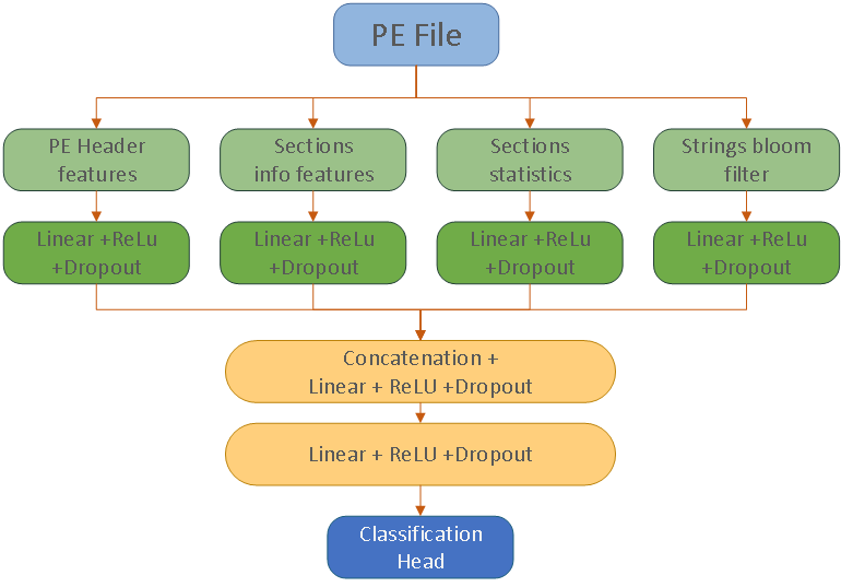
Malware classification neural network
The neural network model works with the following types of features:
- PE Header features – features extracted from PE header, including physical and virtual file size, overlay size, executable characteristics, system type, number of imported and exported functions, etc.
- Section features – the number of sections, physical and virtual size of sections, section c
- Section statistics – various statistics describing raw section data: entropy, byte histograms of different section parts, etc.
- File strings – strings parsed from raw file using special utility. Extracted strings packed into bloom filter
Let’s take a brief look at the bloom filter structure.

Scheme of packing strings into bloom filter structure. Bits related to strings are set to 1
The bloom filter is a bit vector. For each k string n predefined hash functions are calculated. The value of the hash functions determines the position of a bit to be set to 1 in the bloom filter vector. Note that different strings can be mapped to the same bit. In this case the bit remains in the set position (equal to 1). This way we can pack all file strings into a vector of a fixed size.
We trained the aforementioned neural network on approximately 300 million files – half of them benign, the other half malware. The classification quality of this network is displayed in the ROC curve. The X-axis shows the false positive rate (FPR) in logarithmic scale, while the Y-axis corresponds to the true positive rate (TPR) – the detection rate for all the malware files.

ROC curve for trained malware detector
In our company, we focus on techniques and models with very low false positive rates. So, we set a threshold for a 10-5 false positive rate (we rate 1 false positive as 100 000 true detections). Using this threshold, we detected approximately 60% of the malware samples from our test collection.
Adversarial attack algorithm
To attack the neural network, we use the gradient method described in “Practical black-box attacks against machine learning“. For a malware file we want to change the score of the classifier to avoid detection. To do so, we calculate the gradient for the final NN score, back-propagate it through all the NN layers to the file features. The main difficulty of creating an adversarial PE is saving the functionality of the original file. To achieve this, we define a simple strategy. During the adversarial attack we only add new sections, while existing sections remain intact. In most cases these modifications don’t affect the file execution process.
We also have some restrictions for features in the new sections:
- Different size-defining features (related to file/section size, etc.) should be in the range from 0 to some not very large value.
- Byte entropy and byte histograms should be consistent. For example, the values in a histogram for a buffer with the size S should give the value S when combined.
- We can add bits to the bloom filter, but can’t remove them (it is simple to add new strings to the file, but difficult to remove).
To satisfy these restrictions we use an algorithm similar to the one described in “Deceiving end-to-end deep learning malware detectors using adversarial examples” but with some modifications (described below). Specifically, we move the “fix_restriction” step into the “while” loop and expanded the restrictions.

Here dF(x,y)⁄dx is the gradient of the model output by features, fix_restrictions projects features to the aforementioned permitted value area, is the step size.
The adversarial-generating loop contains two steps:
- We calculate gradient of model score by features, and add to the feature vector x in the direction of the gradient for all non-bloom features.
- Update the feature vector x to meet existing file restrictions: for example, put integer file features into the required interval, round them.
For bloom filter features we just set up one bit corresponding to the largest gradient. Actually, we should also find the string for this bit and set up other bits corresponding to it. However, in practice, this level of precision is not necessary and has almost no effect on the process of generating adversarial samples. For simplicity, we will skip the addition of other corresponding string bits in further experiments.
White-box attack
In this section we investigate the effectiveness of the algorithm for the white-box approach. As mentioned above, this scenario assumes the availability of all information about the model structure, as is the case when the detector is deployed on the client side.
By following the algorithm of adversarial PE generation, we managed to confuse our classification model for about 89% of the malicious files.

Removed detection rate. X-axis shows the number of steps in algorithm 1; Y-axis shows the percentage of adversarial malicious files that went undetected by the NN classifier (while their original versions were detected).
Thus, it is easy to change files in order to avoid detection by our model. Now, let us take a closer look at the details of the attack.
To understand the vulnerabilities of our NN we implement the adversarial algorithm for different feature types separately. First, we tried to change string features only (bloom filter). Doing so confuses the NN for 80% of the malware files.

Removed detection rate for string changing only
We also explore which bits of the bloom filter are often set to 1 by the adversarial algorithm.
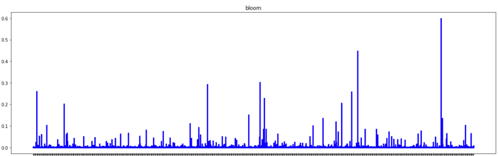
The histogram of bits, added by the adversarial algorithm to the bloom filter. Y-axis corresponds to the ratio of files that the current bit is added to. A higher rate means that bit is important for decreasing the model score
The histogram shows that some bits of the bloom filter are more important for our classifier, and setting them to 1 often leads to a decrease in the score.
To investigate the nature of such important bits we reversed the popular bits back to the string and obtained a list of strings likely to change the NN score from malware to benign:
|
1 2 3 4 5 6 7 8 9 |
Pooled mscoree.dll CWnd MessageBoxA SSLv3_method assembly manifestVersion="1.0" xmlns="urn… SearchPathA AVbad_array_new_length@std Invalid color format in %s file SHGetMalloc Setup is preparing to install [name] on your computer e:TScrollBarStyle{ssRegular,ssFlat,ssHotTrack SetRTL VarFileInfo cEVariantOutOfMemoryError vbaLateIdSt VERSION.dll GetExitCodeProcess mUnRegisterChanges ebcdic-Latin9--euro GetPrivateProfileStringA XPTPSW cEObserverException LoadStringA fFMargins SetBkMode comctl32.dll fPopupMenu1 cTEnumerator<Data.DB.TField cEHierarchy_Request_Err fgets FlushInstructionCache GetProcAddress NativeSystemInfo sysuserinfoorg uninstallexe RT_RCDATA textlabel wwwwz |
We also tried to attack the model to force it to misclassify benign files as malware (inverse problem). In this case, we obtained the following list:
|
1 2 3 4 5 6 7 8 |
mStartTls Toolhelp32ReadProcessMemory mUnRegisterChanges ServiceMain arLowerW fFTimerMode TDWebBrowserEvents2DownloadCompleteEvent CryptStringToBinaryA VS_VERSION_INFO fFUpdateCount VirtualAllocEx Free WSACreateEvent File I/O error %d VirtualProtect cTContainedAction latex VirtualAlloc fFMargins set_CancelButton FreeConsole ntdll.dll mHashStringAsHex mGetMaskBitmap mCheckForGracefulDisconnect fFClientHeight mAddMulticastMembership remove_Tick ShellExecuteA GetCurrentDirectory get_Language fFAutoFocus AttributeUsageAttribute ImageList_SetIconSize URLDownloadToFileA CopyFileA UPX1 Loader |
These sets of “good” and “bad” strings look consistent and plausible. For instance, the strings ‘MessageBoxA’ and ‘fPopupMenu1’ are actually often used in benign files. And vice versa, strings like ‘Toolhelp32ReadProcessMemory’, ‘CryptStringToBinaryA’, ‘URLDownloadToFileA’ and ‘ShellExecuteA’ look suspicious.
We also attempted to confuse our model using only binary sections statistics.
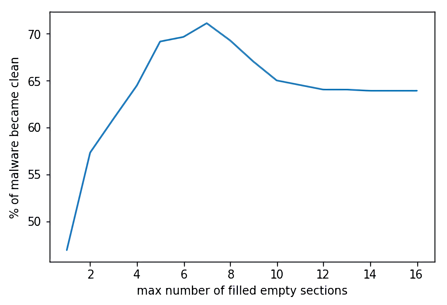
Removed detection rate for section added, without bloom features. X-axis corresponds to the number of added sections, Y-axis to the percentage of malware files that become “clean” during adversarial attacks
The graph shows that it is possible to remove detection for about 73% of malware files. The best result is achieved by adding 7 sections.
At this point, the question of a “universal section” arises. That is, a section that leads to the incorrect classification and detection removal of many different files when added to them. Taking this naïve approach, we simply calculated mean statistics for all sections received during the adversarial algorithm and created one “mean” section. Unfortunately, adding this section to the malware files removes just 17% of detections.

Byte histogram of “mean” section: for its beginning and ending. X-axis corresponds to the byte value; Y-axis to the number of bytes with this value in the section part
So, the idea of one universal section failed. Therefore, we tried to divide the constructed adversarial section into compact groups (using the l2 metric).

Adversarial sections dendrogram. Y-axis shows the Euclidian distance between sections statistics
Separating the adversarial sections to clusters, we calculated a “mean” section for each of them. However, the detection prevention rate did not increase rapidly. As a result, in practice, only 25-30% of detection cases can be removed by adding such “universal mean sections”.

The dependence of the removed detection share on the number of clusters for “mean” sections computation
The experiments showed that we do not have a “universal” section for making a file look benign for our current version of NN classifier.
Gray-box attack
All previous attacks were made with the assumption that we already have access to the neural network and its weights. In real life, this is not always the case.
In this section we consider a scenario where the ML model is deployed in the cloud (on the security company’s servers), but features are computed and then sent to the cloud from the user’s machine. This is a typical scenario for models in the cybersecurity industry because sending user files to the company side is difficult (due to legal restrictions and traffic limitations), while specifically extracted features are small enough for forwarding. It means that attackers have access to the mechanisms of feature extraction. They can also scan any files using the anti-malware product.
We created a number of new models with different architectures. To be precise, we changed the number of fully connected layers and their sizes in comparison with the original model. We also collected a large collection of malware and benign files that were not in the original training set. Then we extracted features from the new collection – this can be done by reversing the code of the anti-malware application. Then we labeled the collection in two different ways: by the full anti-malware scan and using just the original model verdicts. To clarify the difference, with the selected threshold the original model detects about 60% of malware files compared to the full anti-malware stack. These models were trained on the new dataset. After that the adversarial attack described in previous sections was implemented for proxy models. The resulting adversarial samples built for the proxy model were tested on the original one. Despite the fact that the architectures and training datasets of the original and proxy models were different, it turned out that attacks on the proxy model can produce adversarial samples for the original model. Surprisingly, attacking the proxy model could sometimes lead to better attack results.
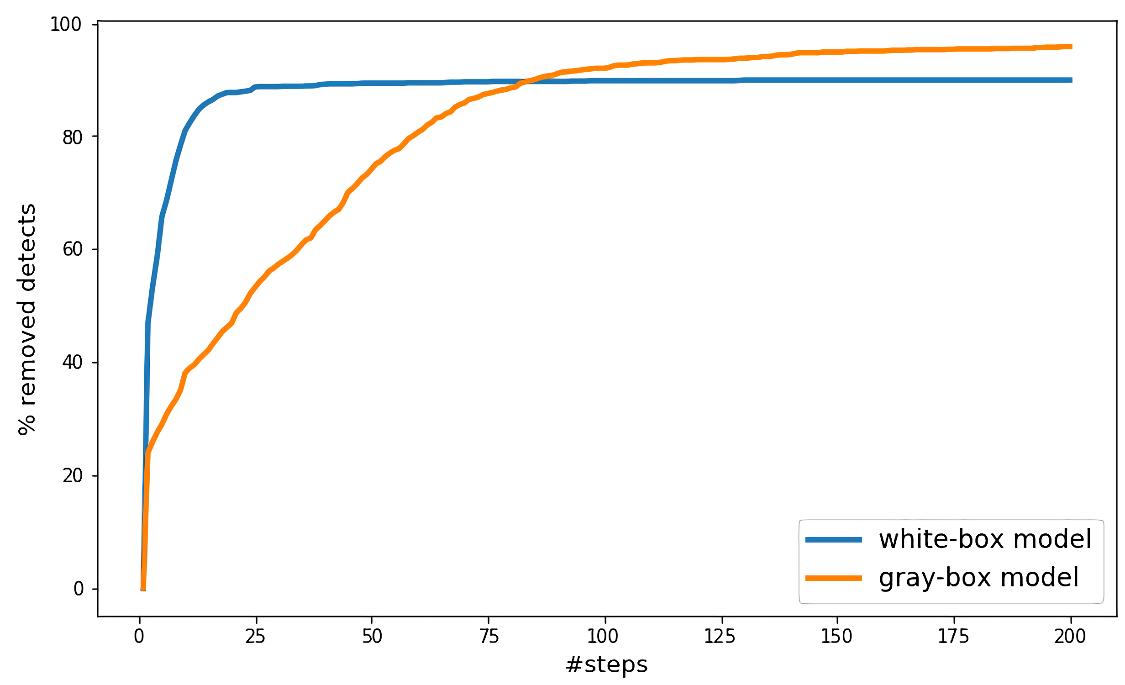
Gray-box attack results compared to white-box attack. Y-axis corresponds to the percentage of malware files with removed detections of the original model. The effectiveness of the gray-box attack in this case is better than that of the white-box attack.
The experiment shows that a gray-box attack can achieve similar results to the white-box approach. The only difference is that more gradient steps are needed.
Attack transferability
We don’t have access to the machine learning models of other security companies, but we do have reports[vi] of gray-box and white-box adversarial attacks being successful against publicly available models. There are also research papers[vii] about the transferability of adversarial attacks in other domains. Therefore, we presume that product ML detectors of other companies are also vulnerable to the described attack. Note that neural networks are not the only vulnerable machine learning type of model. For example, another popular machine learning algorithm, gradient busting, is also reported[viii] to have been subjected to effective adversarial attacks.
Adversarial attack protection
As part of our study, we examined several proposed algorithms for protecting models from adversarial attacks. In this section, we report some of the results of their impact on model protection.
The first approach was described in “Distillation as a defense to adversarial perturbations against deep neural networks“. The authors propose to train the new “distilled” model based on the scores of the first model. They show that for some tasks and datasets this method reduces the effectiveness of gradient-based adversarial attacks. Unfortunately, the idea does not guarantee successful model protection, and in our case, when we trained the model according to the proposed approach, it still turned out to be easily confused by the adversarial algorithm.
We also tried to add noise to data:
- For continuous features we calculated mean and standard deviation values. We added a random number of sections to each file during model training. Then the generated sections parameters were taken from a Gaussian distribution with parameters equal to the aforementioned mean and deviation values.
- For the bloom filter structure, we also added a 5% chance of setting each bit to 1.
The idea behind this method is to try to expand the set of potential file sections, making the network more stable and resistant to attacks that add sections to the end of a file. However, this method was not effective either.
We also tried the protection approach described in “Detecting adversarial samples from artifacts“. In many cases, neural network layers contain a dropout mechanism. A dropout is a layer that randomly replaces features from a previous layer with zeros. The idea of the paper is to enable a dropout in the inference stage (while it is usually disabled because the dropout layer mechanism produces a level of randomness and noise in predictions for the same objects), and calculate the score multiple times for each file. Enabling dropout layers leads to slightly different scores for each run, so we get a score distribution. These distributions, according to the authors, have standard deviation values for adversarial samples that are higher than for usual samples. We tried this approach, computing standard deviations of scores for adversarial malware and original malware files. Remarkably, the standard deviations of the adversarial scores appeared to be significantly higher than the deviations of the initial file scores.

Standard deviation distribution for adversarial and initial sample model scores
With this difference we can, for example, detect 50% of adversarial samples with initial sample misclassification of around 10%, with a threshold.

X-axis shows the share of original samples detected as adversarial; Y-axis shows the share of detected adversarial samples
The other approach proposes the use of monotonic networks (see “Monotonic Networks” and “Monotonic models for real-time dynamic malware detection“). The principle behind this method is to create a neural network with positive layer weights and monotonic activation functions. Such models will, by design, be resistant to the addition of new sections and strings, and any addition will simply increase the model detection score, making the attack described in this article impracticable.
Adversarial attack difficulties in the real world
Currently, there is no approach in the field of machine learning that can protect against all the various adversarial attacks, meaning methods that rely heavily on ML predictions are vulnerable. Kaspersky’s anti-malware solution provides a complex multi-layered approach. It contains not only machine learning techniques but a number of different components and technologies to detect malicious files. First, detection relies on different types of features: static, dynamic or even cloud statistics. Complex detection rules and diverse machine learning models are also used to improve the quality of our products. Finally, complex and ambiguous cases go to the virus analysts for further investigation. Thus, confusion in the machine learning model will not, by itself, lead to misclassification of malware for our products. Nevertheless, we continue to conduct research to protect our ML models from existing and prospective attacks and vulnerabilities.
[i] Goodfellow, Ian J., Jonathon Shlens, and Christian Szegedy. “Explaining and harnessing adversarial examples.” arXiv preprint arXiv:1412.6572 (2014).
[ii] Brown, Tom B., et al. “Adversarial patch.” arXiv preprint arXiv:1712.09665 (2017).
[iii] Demetrio, Luca, et al. “Functionality-preserving black-box optimization of adversarial windows malware.” IEEE Transactions on Information Forensics and Security (2021).
[iv] Sharif, Mahmood, et al. “Optimization-guided binary diversification to mislead neural networks for malware detection.” arXiv preprint arXiv:1912.09064 (2019).
[v] Kolosnjaji, Bojan, et al. “Adversarial malware binaries: Evading deep learning for malware detection in executables.” 2018 26th European signal processing conference (EUSIPCO). IEEE, 2018;
Kreuk, Felix, et al. “Deceiving end-to-end deep learning malware detectors using adversarial examples.” arXiv preprint arXiv:1802.04528 (2018).
[vi] Park, Daniel, and Bülent Yener. “A survey on practical adversarial examples for malware classifiers.” arXiv preprint arXiv:2011.05973 (2020).
[vii] Liu, Yanpei, et al. “Delving into transferable adversarial examples and black-box attacks.” arXiv preprint arXiv:1611.02770 (2016).
Tramèr, Florian, et al. “The space of transferable adversarial examples.” arXiv preprint arXiv:1704.03453 (2017).
[viii] Chen, Hongge, et al. “Robust decision trees against adversarial examples.” International Conference on Machine Learning. PMLR, 2019.
Zhang, Chong, Huan Zhang, and Cho-Jui Hsieh. “An efficient adversarial attack for tree ensembles.” arXiv preprint arXiv:2010.11598 (2020).
How to confuse antimalware neural networks. Adversarial attacks and protection


Imre Kaliczi
Very good, summary of ML based methods.